State Space Models lack sequence-crossing

date

Mar 2, 2024

slug

ssm_review

status

Published

summary

My opinions on SSMs

Opinion

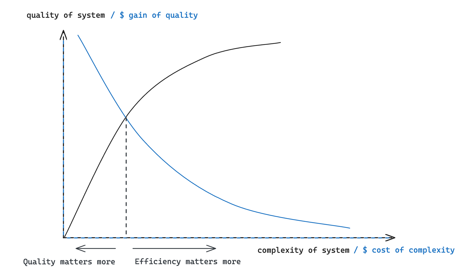
Every architecture contains some implicit trade-offs. My impression is SSMs are a good sequential architecture for modalities where interactions within a sequence matters less than a good compression of past states. However, it might not be the best architecture if the following 2 conditions are met:

The marginal gain of additional compression quality outweighs the efficiency loss.

The way a task depends on past history varies a lot (the definition of “a lot” will become clearer later).

The 1st condition is fairly self-explanatory and is generally true for complicated deep learning tasks (chatbot, self-driving), at least for the time being, and especially true for areas that are yet to be solved.

An illustration of quality-efficiency trade-off

The 2nd condition is more subtle, because what does “the way a task depends on past history” actually mean? Before attempting to answer this question, here’s why I think it matters for SSM models.

But even before that, let’s do a quick recap of state space models are.

SSM Models

When I refer to SSM models, I’m not referring to the classical state space models used in a control context or a quantitative finance context, but rather SSM in the context of sequential neural networks.

Literature roadmap of recent State Space neural network Model architectures

The above is literature roadmap of recent SSM architectures. The are some terrific detailed explanation on what they are:

The Annotated S4 dives deep into S4 and explained the inner workings of S4.

A Visual Guide to Mamba and State Space Models explained, visually, what mamba does.

From Deep to Long Learning? where the authors themselves gave a good account of the development of H3 and Hyena.

In short, SSM is the following process that models state changes of a system

(The above is only for discrete problem, similar formulation for continuous time; Also I’m neglecting the discretization step here for illustration purpose)

There’re many properties to this model, and its usefulness is immense in the field of control, signal processing, time series application, etc.

History preserving

Just by laying out the equations above does not guarantee a good compression of past history. The magic of SSMs comes from the theory of approximation theory, and in particular, orthogonal polynomials.

Consider a scale value that varies with sequence , i.e.,

Suppose we want to approximate the history with a limited number of numbers , one way to achieve it is to let each correspond to a “basis function” and let

The approximation error is therefore defined as

The weighting function is added to further generalize the discussion. Expanding the error, one obtains

In practice, we don’t have to limit ourselves to integrating from to . This motivates defining the inner product in the function space

The approximation error can be further rewritten as

Now, wouldn’t it be nice if we can eliminate some of the terms here? In fact, we can do exactly that with orthogonal polynomials.

Orthogonal Polynomials

Orthogonal polynomials have the property that they are orthogonal to each other under the inner product definition, i.e.,

One example would be the Legendre polynomials, which is defined over with , and is of the following forms

(note: there’s one unique set of OPs for any weight function for any given interval)

With this property, the approximation error simplifies to (the 3rd term disappears)

To simplify it further, let’s define the constant in a meaningful way by taking the gradient of with respect to and set it to 0

The above gives us a way to combine a set of orthogonal polynomials to achieve minimum approximation error with respect to any function .

Make the weight time-dependent

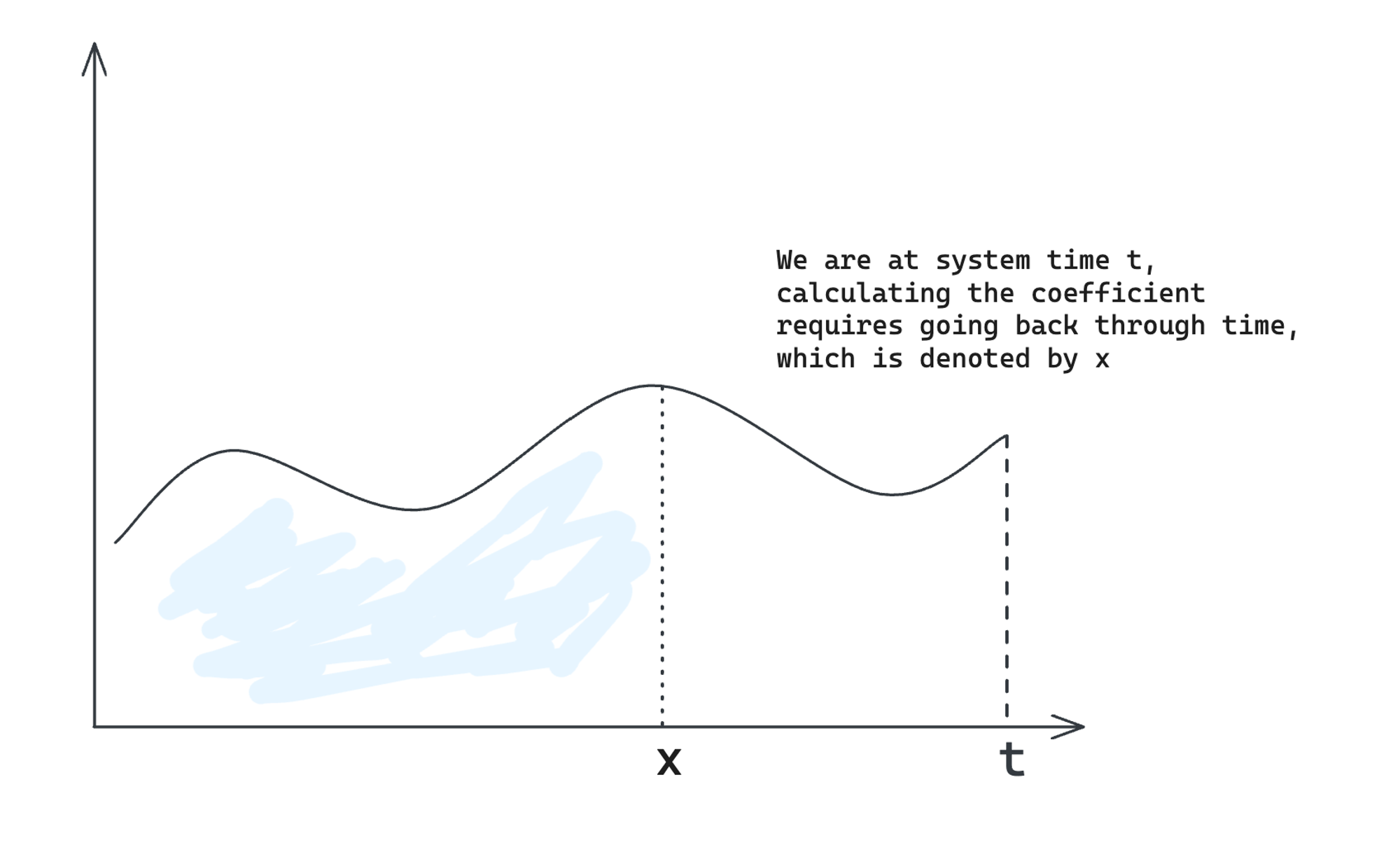
Now, what if the weighting function is also time dependent (changes over time)? Instead of , we have . This leads to a more complicated system where everything should be defined with respect to another time. To save you some time, this leads to the following equation for the “minimization coefficient”

where is the basis OP used in the system, is a scaling function to increase the generality of the argument, and is a normalization term caused by , is the time-varying weighting function.

The difference between and is plotted below.

Now, why on earth would we want to do this? We want to do this because we want to take the derivative of with respect to , and hopefully derive a SSM out of it. We can do exactly that

The beauty here is that and can both be expressed in close-form and related back to themselves, which means we get an ODE out of this!

Once an ODE is obtained, we can structure it to form an SSM. Note that the precise form of SSM depends on what weighting function/OP we use. Different choice of weighting function represents how we weight the history.

Here’s an example of the explicit form of SSM, for the Laguerre polynomials

Problem?

After defining the SSM in the continuous domain, one needs to discretize it and turn it into actual architecture and code. However, here I want to focus on 2 properties of SSM:

💡

1. The way that evolves by itself is time invariant 2. The way affects is additive

(here I’m abusing notations by using and interchangeably, and using for )

To elaborate a bit, it means

Without external input, this is a deterministic linear system (by design), and it’s much computationally easier to compute a linear system (i.e., convolution can be applied)

The expressiveness of the system is bound by linearity

To see why the 2nd point is true, we can expand the system equation and obtain

where it’s clear can only affect the system state in linear fashion, if and are fixed. Also, if and are fixed, is also affected by in a linear fashion.

Lack of non-linearity

It’s clear that such a system, while might be desirable for system control, is not ideal to express a complicated system that is non-linear. And it’s hard to argue that tasks like language modeling will be a linear system. In the most recent architectures (such as Mamba), this lack of expressiveness is addressed by

replacing with

replacing with

replacing with

Therefore, the governing equation is replaced by

where we can fold the input further into and without loss of generality, and obtain

Similarly, we can expand the system again and obtain

Although this is technically a non-linear system as long as or or is non-linear (for example, ), this modeling does not involve any sequence-crossing terms like .

This, in my opinion, hugely impacts the expressiveness of the system because the lack of sequence-cross in sequential modeling is similar to the lack of feature-crossing in tabular modeling, which will result in low sample efficiency.

Mamba to the rescue?

In the Mamba paper, the authors (I’d argue partially) addressed this issue by:

inserting a convolution layer before , but I don’t see how that will fundamentally change the picture, because and will not interact with each other if their sequential distance is larger than the convolution kernel size.

having more layers so and can interact with each other at a higher layer, but this does not change the fact that on a given layer, no cross-sequence interaction can happen.

creating a gating layer so that an explicit sequence-crossing layer is added to the output , i.e.,

which technically makes sequence-crossing possible. This is similar to GRU and LSTM. The additional expressiveness of such a gating mechanism, one can argue, is much less that attention, because the gate itself does not contain sequence-crossing terms.

Intuition

By turning the linear SSM into an non-linear SSM, and adding these 3 additional modifications, SSM seem to perform well across many modalities (arguments can be made on the details of some of these experiment results, such as the extremely low vocab size used in the induction head task).

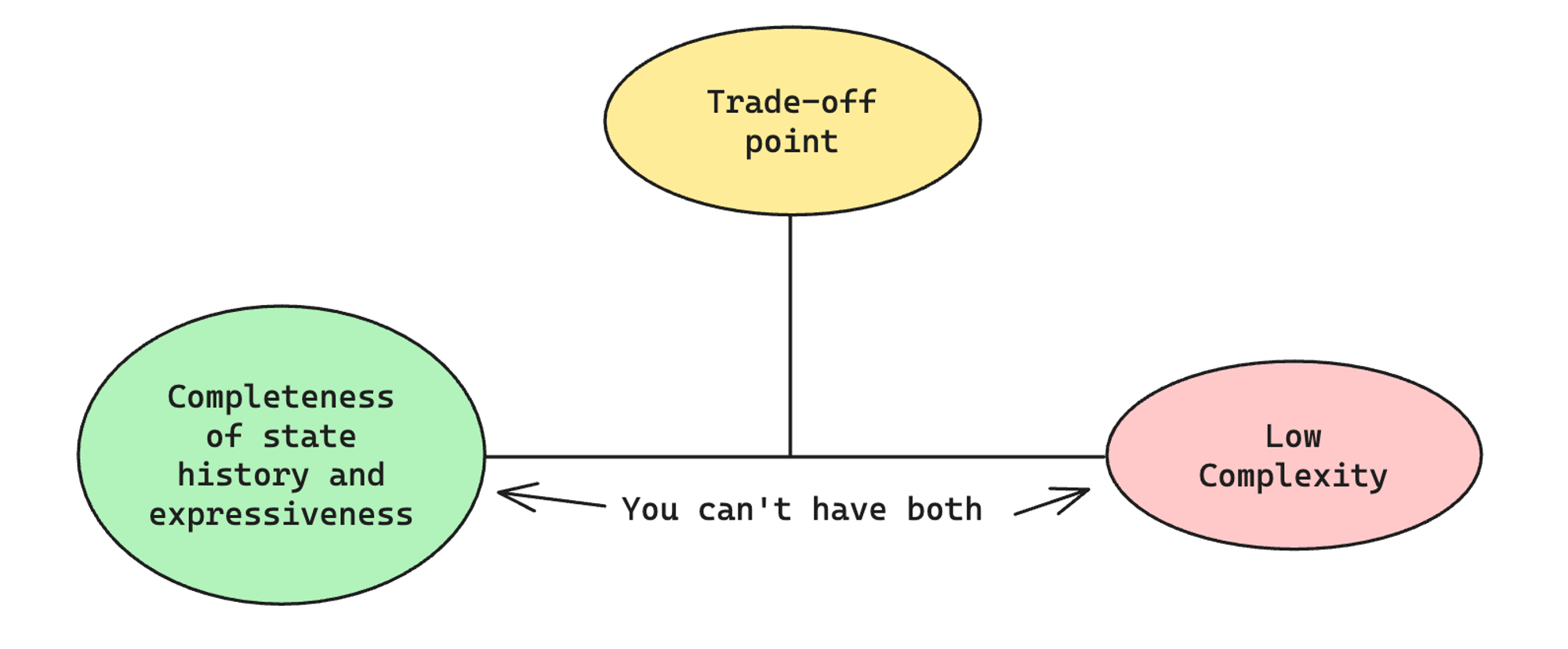
However, a pattern has emerged through the evolution of SSM models where we started off with a beautiful mathematical model (a unified compression scheme) that has theoretical guarantees on approximation error and implementation efficiency. However, due to our limited understanding of the expressiveness required for complicated domains like language, an iterative approach must be taken to move the trad-off point (illustrated below) towards one that uses the minimum complexity to achieve the required expressiveness and completeness.

The question then becomes “is transformer already at the best trade-off point”? For most domains?

I have no idea.

References

[1] Gu, A., & Dao, T. (2023). Mamba: Linear-Time Sequence Modeling with Selective State Spaces (arXiv:2312.00752)

[2] Chihara, T. S. (2011). An introduction to orthogonal polynomials. Courier Corporation.

[3] Olsson, Catherine, et al. "In-context learning and induction heads." arXiv preprint arXiv:2209.11895 (2022).